Code
# Library Imports
library(tidyverse)
library(readr)
library(ggplot2)
library(dplyr)The “2015 Street Tree Census - Tree Data” dataset is a comprehensive collection of information on New York City’s street trees, compiled by the NYC Department of Parks & Recreation in collaboration with volunteers and partner organizations between May 2015 and October 2016. Representing the largest citizen science initiative in the city’s history, the dataset includes detailed attributes for 666,134 recorded trees across New York City’s five boroughs.
Source : 2015 Street Tree Census - Tree Data
Data Collection :
The data was collected by trained volunteers and NYC Parks staff, using standardized protocols to ensure consistency. Each tree’s attributes, including species, diameter, health status, and geographic location, were recorded during the census. The data collection process also involved visual inspections and field surveys to gather accurate information on tree conditions and their interactions with surrounding infrastructure.
Data Format and Structure:
The data is presented in a tabular format, with each row representing an individual tree and columns detailing its attributes. Key attributes include:
Dimensions and Scope:
The dataset comprises 166,134 records and 45 columns, each corresponding to an individual street tree. It offers a rich combination of categorical and numerical variables suitable for diverse analytical approaches. Its spatial information enables geospatial analyses, such as examining tree distribution patterns across neighborhoods and boroughs. This richness makes the dataset particularly well-suited for exploratory data analysis, allowing us to uncover trends and insights relevant to urban forestry management.
Frequency of Update :
The dataset is static, representing a one-time snapshot of the NYC street trees as they existed during the census period (2015–2016). It does not receive updates and serves as a historical record.
Importing the Data :
The dataset will be imported using R’s read.csv() function to handle its large size efficiently.
# Library Imports
library(tidyverse)
library(readr)
library(ggplot2)
library(dplyr)# Importing the data, we are using partial data due to computational limits.
tree_data <- read_csv("../2015_Street_Tree_Census_-_Tree_Data_20241120.csv", n_max = 266134)# storing the data with missing values in a variable
tree_data_with_na <- tree_data |>
mutate(across(everything(), ~ ifelse(is.na(.) | . == "" | . == " " | . == "None", NA, .)))
# Step 1: Count NA values in each column
na_counts <- tree_data_with_na %>%
summarise(across(everything(), ~ sum(is.na(.)))) %>%
t() %>%
as.data.frame()
# Add column names for clarity
colnames(na_counts) <- c("NA_Count")
na_counts$Column <- rownames(na_counts)
rownames(na_counts) <- NULL
# Step 2: Calculate total rows and convert counts to percentages
total_rows <- nrow(tree_data)
na_counts <- na_counts %>%
mutate(Percentage = (NA_Count / total_rows) * 100)
# Step 3: Filter out columns with no NA values
na_counts_filtered <- na_counts %>%
filter(NA_Count > 0)
# Step 4: Plot NA percentages for remaining columns
ggplot(na_counts_filtered, aes(x = reorder(Column, -Percentage), y = Percentage)) +
geom_bar(stat = "identity", fill = "steelblue", color = "black", width = 0.7) +
geom_text(aes(label = paste0(round(Percentage, 1), "%")),
vjust = -0.5, size = 4, color = "black") +
theme_minimal() +
labs(
title = "Percentage of Missing Values Across Columns Containing NA Values",
x = "Columns",
y = "Percentage of Missing Values"
) +
scale_y_continuous(labels = scales::percent_format(scale = 1)) +
theme(
plot.title = element_text(hjust = 0.5, size = 14, face = "bold"),
axis.text.x = element_text(angle =35, hjust = 1, size = 10),
axis.text.y = element_text(size = 10),
axis.title.x = element_text(size = 12, face = "bold"),
axis.title.y = element_text(size = 12, face = "bold")
)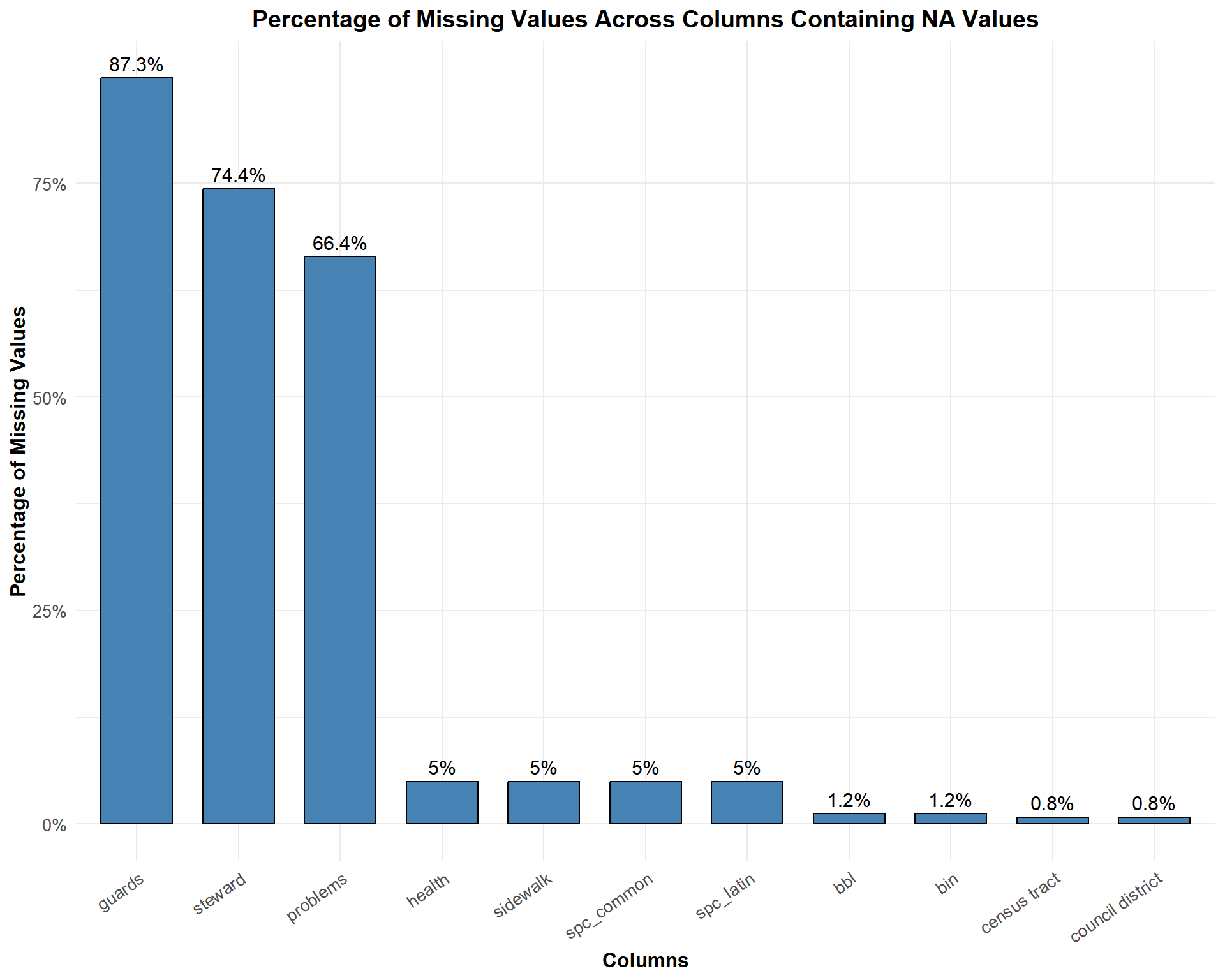
High Missing Value Columns
guards: With 87.3% missing values, this column has the highest rate of missingness. The data on tree guards might not have been consistently collected, possibly because it was optional or difficult to assess during the survey.steward: At 74.4% missing values, this column reflects limited data availability on tree stewardship. This may be due to a lack of reporting or complexity in identifying individuals or groups responsible for tree care.problems: This column has 66.4% missing values. It indicates incomplete data on issues affecting the trees, which could result from challenges in identifying or documenting tree-related problems.Moderate and Low Missing Value Columns
spc_common, spc_latin, health, sidewalk: These columns have around 50% missing values. These fields likely had better data collection protocols but still show gaps, potentially due to oversight or difficulty in identifying specific attributes (e.g., species or tree health conditions).bbl, bin, census tract, council district: These columns exhibit very low missing values (less than 2%). These administrative or geographic fields were likely easier to document consistently, but small gaps might have occurred due to technical issues or incomplete records.Columns with No Missing Values
# Step 1: Convert all columns to character type (except row identifier)
tree_data_char <- tree_data_with_na %>%
  mutate(across(everything(), as.character))

# Step 2: Add a row identifier
tree_data_char <- tree_data_char %>%
  mutate(row = row_number())

# Step 3: Reshape data into long format, excluding the `row` column
na_heatmap_data <- tree_data_char %>%
  pivot_longer(cols = -row, names_to = "Column", values_to = "Value") %>%
  mutate(Missing = is.na(Value) | Value == "" | Value == "None")

# Step 4: Plot the heatmap
ggplot(na_heatmap_data, aes(x = Column, y = row, fill = Missing)) +
  geom_tile() +
  scale_fill_manual(values = c("TRUE" = "red", "FALSE" = "white")) +
  theme_minimal() +
  labs(
    title = "Heatmap of Missing Values (All Columns)",
    x = "Columns",
    y = "Rows",
    fill = "Missing"
  ) +
  theme(
    axis.text.x = element_text(angle = 90, hjust = 1),
    axis.text.y = element_text(size = 7),
    plot.title = element_text(hjust = 0.5))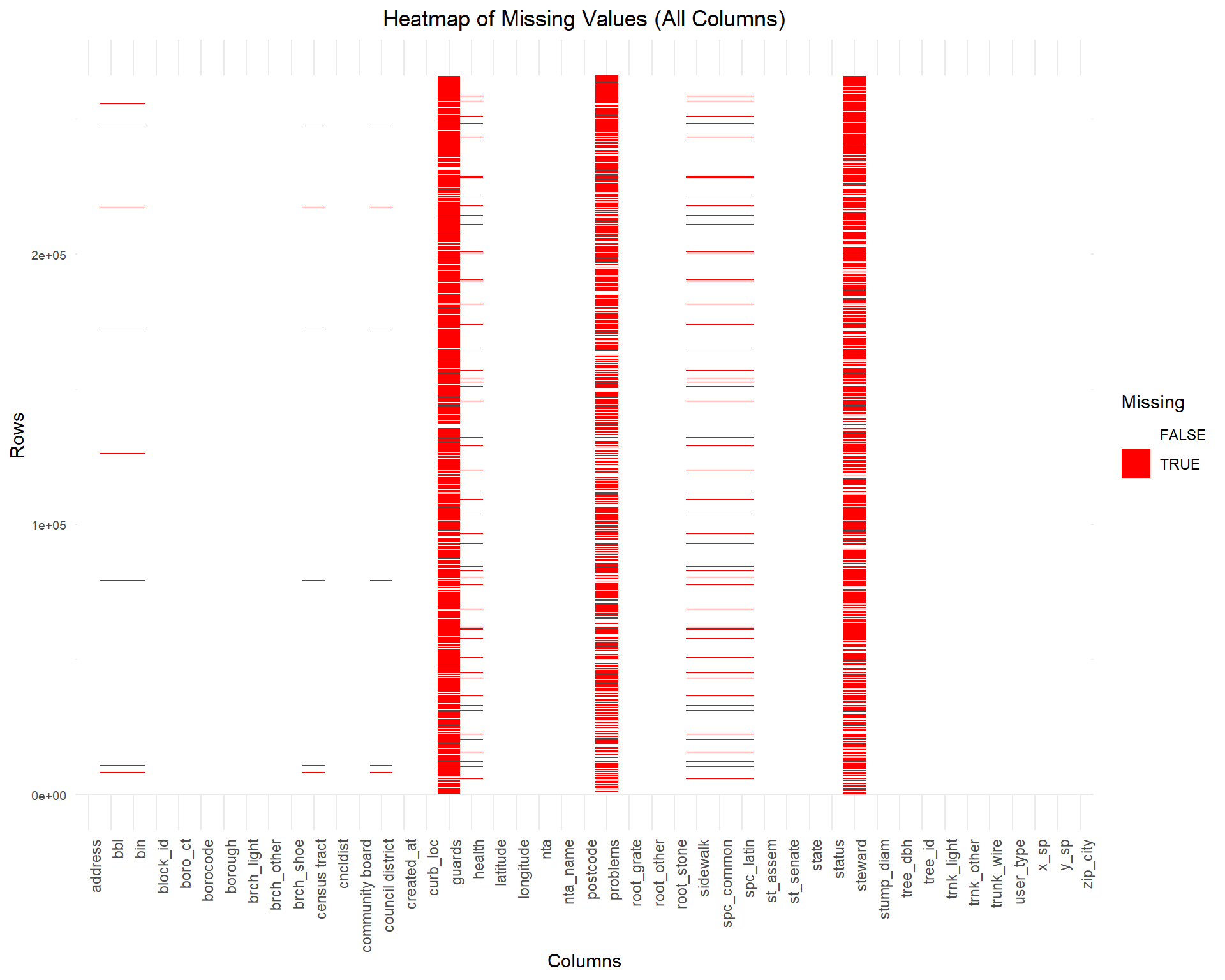
guards, steward, and problems (frequent red blocks).bbl, bin, and census tract have very few missing values, shown by minimal red blocks.# Step 1: Convert all columns to character type (except row identifier)
tree_data_char <- tree_data_with_na %>%
mutate(across(everything(), as.character))
# Step 2: Identify columns with NA values
columns_with_na <- tree_data_char %>%
summarise(across(everything(), ~ sum(is.na(.) | . == "" | . == "None"))) %>%
select(where(~ . > 0)) %>%
names()
# Step 3: Filter to include only columns with NA values and add row identifier
tree_data_filtered <- tree_data_char %>%
select(all_of(columns_with_na)) %>%
mutate(row = row_number())
# Step 4: Reshape data into long format, excluding the `row` column
na_heatmap_data <- tree_data_filtered %>%
pivot_longer(cols = -row, names_to = "Column", values_to = "Value") %>%
mutate(Missing = is.na(Value) | Value == "" | Value == "None") # Detect missing values
# Step 5: Plot the heatmap
ggplot(na_heatmap_data, aes(x = Column, y = row, fill = Missing)) +
geom_tile() +
scale_fill_manual(values = c("TRUE" = "red", "FALSE" = "white")) +
theme_minimal() +
labs(
title = "Heatmap of Missing Values (Columns with NA Values Only)",
x = "Columns",
y = "Rows",
fill = "Missing"
) +
theme(
axis.text.x = element_text(angle = 90, hjust = 1),
axis.text.y = element_text(size = 7),
plot.title = element_text(hjust = 0.5)
)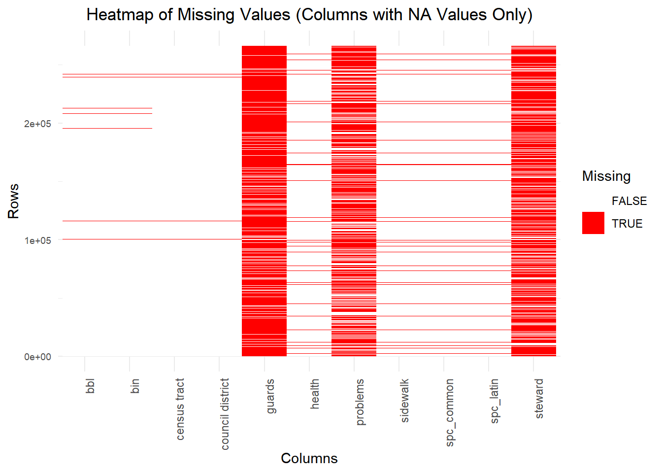
guards and steward exhibit the highest missingness, with red blocks dominating most rows.health, problems, and sidewalk, with scattered red blocks.bbl and bin, have fewer red blocks compared to others.NA in R, while others are explicitly recorded as "None". Additionally, there are instances where missing values are represented as blank strings ("") or blank spaces (" ").guards, steward, problems) may require imputation or exclusion, depending on their importance in the analysis.